This site currently features a complete guide for reconstructing real-world objects using 3D Gaussian Splatting. It walks you through image capture, camera pose estimation, model training, and post-processing, all using open-source tools on Windows.
More tutorials will be added in the future.
1 - From Real Object to 3D Gaussian Splatting Model Using Open-Source Tools
A step-by-step guide for capturing real objects or physical products and reconstructing them on Windows using COLMAP, gsplat, and SuperSplat.
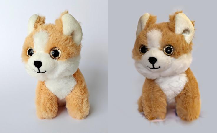
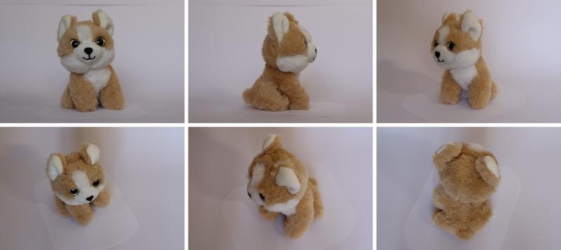
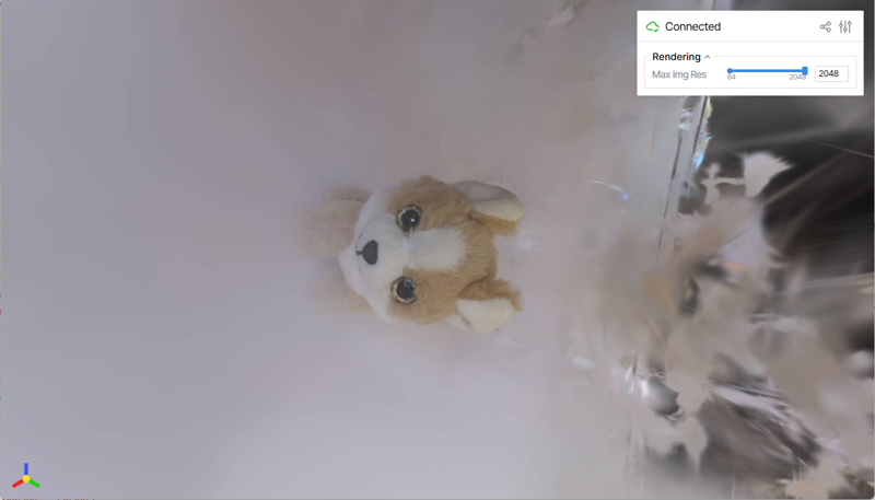
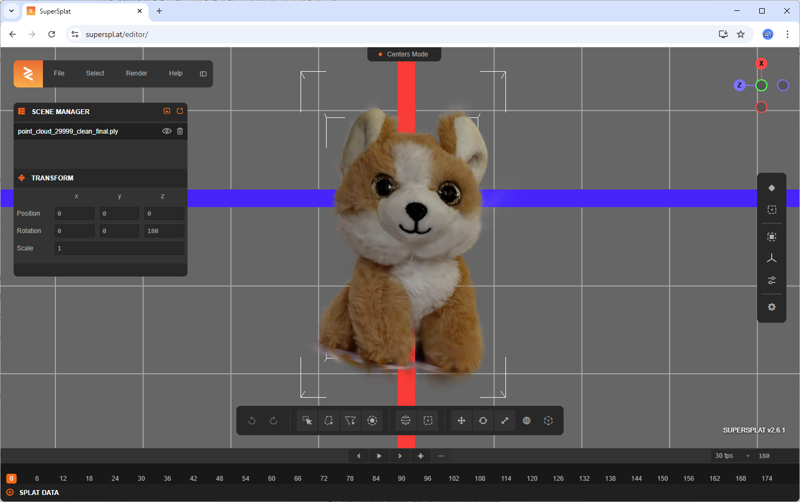
Real-world plush toy (left) and its reconstructed 3D Gaussian Splatting model (right).
Gaussian Splatting is a modern technique for novel view synthesis. It reconstructs scenes by placing thousands of small 3D Gaussians in space and optimizing their appearance to match the input images. This approach is particularly effective at capturing fine and soft details, such as fur or fabric textures, which are often difficult for traditional surface-based methods.
This tutorial demonstrates the complete pipeline using a real plush toy as the subject. It includes the following steps:
Capture input images
Estimate camera poses with COLMAP
Train the model using gsplat
Edit and visualize results with SuperSplat
The example shows how to achieve reproducible results using only open-source tools configured for Windows.
This workflow is especially well-suited for scanning physical products or small real-world objects, making it useful for applications such as product visualization, object digitization, and 3D content creation.
About gsplat
This tutorial uses the gsplat repository for 3D Gaussian Splatting. Compared to the original implementation by the authors (graphdeco-inria/gaussian-splatting), gsplat provides several practical advantages:
Supports faster training, lower memory usage, and large scenes
Includes features such as multi-GPU support, depth rendering, and anti-aliasing
Integrates with the Nerfstudio ecosystem for shared tools and pipelines
Released under the Apache 2.0 license, which allows commercial use
Actively maintained and used by open-source projects
About COLMAP
COLMAP estimates camera poses and generates a sparse reconstruction from input images. These results are used to train the 3D Gaussian Splatting model. The Windows version of COLMAP includes both a graphical interface and command-line tools.
Note: gsplat is part of the Nerfstudio project, which includes a built-in COLMAP wrapper that runs with default parameters. This is often sufficient, but some datasets require custom settings for successful reconstruction. A later section explains how to adjust key parameters when the defaults do not work.
Note: Other tools such as RealityCapture, Agisoft Metashape, or Autodesk ReCap Pro can be used for similar pipelines. This tutorial focuses on free and reproducible workflows using COLMAP.
About SuperSplat
SuperSplat Editor is an open-source, browser-based tool for viewing, editing, and optimizing 3D Gaussian Splatting models. It supports the following tasks:
Inspecting results
Cleaning up artifacts
Cropping and merging models
Performing lightweight edits without retraining
SuperSplat can also be installed as a Progressive Web App (PWA) for faster access and desktop integration.
Windows as the target platform
This tutorial focuses on Windows because it is widely used by beginners, students, and general technical users. While many open-source tools are developed for Linux, Windows users often face additional setup challenges due to platform-specific differences.
Questions about installing and running COLMAP and gsplat on Windows are common in forums, GitHub issues, and online communities. This tutorial provides a clear, step-by-step workflow tailored to Windows to help make modern 3D reconstruction techniques more accessible.
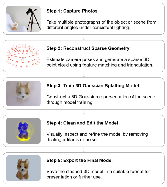
Pipeline overview
This tutorial walks through the full pipeline for building a 3D Gaussian Splatting model from real-world images. The process includes four main stages:
Image capture
Camera calibration and sparse point cloud reconstruction with COLMAP
Model training using gsplat
Final editing and visualization in the SuperSplat viewer
Overview of the 3D Gaussian Splatting pipeline.
The following sections explain each step in detail. You can skip to a specific section if you’re interested only in training, visualization, or another part of the workflow.
1.1 - Installation
This tutorial was developed and tested on Windows 11. Most steps also work on Linux, with some differences that will be addressed in a separate guide.
Recommended environment
For efficient training and reproducibility, use a system with the following configuration:
Hardware
NVIDIA GPU with CUDA support
Software
Windows 11
Git
Miniconda or Anaconda
Microsoft Build Tools for Visual Studio 2022
Python 3.10
CUDA Toolkit 12.6 or a compatible version (install separately)
COLMAP (with CUDA support)
gsplat
SuperSplat
Note: Minor differences in software versions or CUDA drivers may require small adjustments.
Note: The CUDA Toolkit must be installed separately from the GPU driver to enable GPU acceleration. Without it, tools like PyTorch will not detect CUDA support. For instructions and compatibility details, see the CUDA Toolkit documentation.
Tested setup
This tutorial was verified using the following configuration:
Extract the contents of the ZIP file to a convenient location, such as:
C:\Tools\colmap
This tutorial uses <COLMAP_PATH> as a placeholder for the COLMAP installation path. Replace it with the actual path you used.
Launch COLMAP
You can start the COLMAP GUI using either of the following methods:
Option A
Double-click COLMAP.bat in the extracted folder.
Option B
Open Command Prompt and run:
<COLMAP_PATH>\COLMAP.bat gui
Replace <COLMAP_PATH> with the actual installation path.
Verify the installation
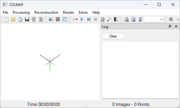
If installed correctly, the COLMAP GUI should open without errors. You should see the main window, as shown below:
Figure 3. COLMAP GUI main window on startup.
Alternative installation methods
This tutorial uses the precompiled Windows release. For other options, including building from source or using package managers on Linux or macOS, refer to the official guide:
https://colmap.github.io/install.html
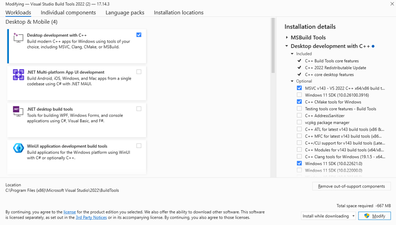
1.1.2 - Installing Microsoft Build Tools
The Microsoft Build Tools for Visual Studio provide the C++ compiler and related tools required to build C++ projects on Windows. This setup is necessary to compile gsplat from source.
If the compiler is configured correctly, you will see the same output as in the previous option.
1.1.3 - Installing gsplat and Preparing for Training
Verify that CUDA Toolkit is installed
Before installing PyTorch or building gsplat, verify that the CUDA Toolkit is installed and accessible. In Command Prompt, run:
nvcc --version
If installed correctly, you should see output similar to:
nvcc: NVIDIA (R) Cuda compiler driver
Copyright (c) 2005-2024 NVIDIA Corporation
Built on Fri_Jun_14_16:44:19_Pacific_Daylight_Time_2024
Cuda compilation tools, release 12.6, V12.6.20
Build cuda_12.6.r12.6/compiler.34431801_0
If the command is not recognized or no version is shown, install the CUDA Toolkit from the NVIDIA website. Older versions are available from the CUDA Toolkit archive.
Open a developer-enabled terminal
To build gsplat, use a terminal with the Visual C++ environment initialized.
Replace <DATA_PATH> and <OUTPUT_PATH> with valid paths. If everything is set up correctly, the script should start and display a training progress bar.
Known issue on Windows: pycolmap binary parsing error
On Windows, you might encounter the following error when running the training script:
Error with pycolmap:
...
num\_cameras = struct.unpack('L', f.read(8))\[0]
This error is caused by mismatched struct unpacking logic in the Windows version. As of this writing, the fix has not yet been merged into the official pycolmap repository. For details, see the related pull request: https://github.com/rmbrualla/pycolmap/pull/2
To work around the issue, uninstall the original package and install a patched version from a community fork:
gsplat supports a variety of input formats using the data processing mechanisms provided by Nerfstudio. This tutorial uses a set of individually captured images as input.
Data capture practices may vary depending on the scene type. Outdoor environments, indoor spaces, human subjects, and small objects each benefit from different techniques. However, the following general guidelines apply in most scenarios and help improve the quality of 3D Gaussian Splatting results.
General guidelines
Use consistent, soft lighting
Illuminate the scene with even, diffuse light to reduce shadows and reflections. Avoid harsh directional light, which can create noise and degrade reconstruction quality.
Capture high-quality still images
Still photos typically produce better results than video frames due to reduced motion blur and more stable exposure. If using video, record at a high frame rate (at least 60 FPS) under steady lighting.
Maintain sufficient image overlap
Each image should overlap with adjacent views by about 20 to 30 percent. Overlap is essential for feature matching in Structure-from-Motion (SfM). Video often provides this overlap automatically.
Ensure parallax by moving the camera
Change the camera’s physical position between shots. Avoid rotating in place without translation, as this limits geometric information and may cause pose estimation to fail.
Keep camera settings fixed
Use manual focus and fixed focal length to keep camera intrinsics consistent. Disable zoom, autofocus, and auto exposure.
Prevent motion blur and distortion
Use a tripod or stabilizer. Avoid low-light conditions that require long exposures. Check that images are sharp and properly focused.
Include texture-rich surfaces
Scenes should have enough texture, edges, or detail to enable reliable feature detection. Flat, uniform, or glossy surfaces may reduce SfM effectiveness.
Keep the scene static
Do not allow movement during capture. Objects, people, or lighting changes can interfere with pose estimation.
Choose an appropriate image resolution
Higher resolutions improve detail but increase memory usage and training time. Choose a resolution that balances quality and performance.
Capture enough views
For small objects or scenes, 100 to 250 well-aligned images is a good starting point. Larger or full 360-degree models require more coverage. Make sure areas like the underside of objects are not missed.
Use multi-camera rigs when helpful
A multi-camera setup can speed up capture by recording multiple views at once. This is useful for dynamic scenes or time-limited sessions.
About the sample data
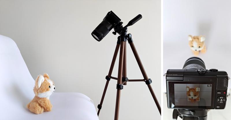
This tutorial uses 84 input images at 3000 × 2000 resolutioncaptured with a Canon M200 camera mounted on a tripod. The plush toy was placed on a chair covered with two stapled 50 × 70 cm sheets of white paper, forming a curved background. An extra sheet underneath allowed for easy rotation of the object during capture, while the camera remained fixed for each donut-shaped sweep.
Photos were taken indoors using only ambient light. Shadows and background elements are visible. This was intentional to simulate real-world conditions and show that good results are still possible without ideal lighting or studio setups. Lighting was uneven and no per-image post-processing was performed. This demonstrates how tools like SuperSplat can help correct brightness and color after training. The goal is to encourage hands-on learning, even with imperfect data.
Note: You can achieve similar results using a modern smartphone, as long as the lighting is adequate and the camera is held steadily.
Note: The plush toy is personally owned and is used here strictly for technical demonstration.
Selected input images used for 3D reconstruction.
Capture setup showing the plush toy, tripod-mounted camera, and curved paper background on a chair (left); live preview of the object on the camera screen during capture (right).
Observation: Gaussian Splatting and fine details
The plush toy was chosen to demonstrate one of the key strengths of 3D Gaussian Splatting: its ability to capture soft, detailed surfaces. Traditional mesh-based pipelines often struggle with materials like fur, resulting in unrealistic or incomplete geometry. In contrast, representing the scene as a set of 3D Gaussians helps preserve fine textures and subtle variations more effectively.
1.3 - Estimate Camera Parameters and Sparse Point Cloud with COLMAP
COLMAP processes the input images to estimate camera intrinsics and extrinsics. It also generates a sparse point cloud, which serves as the geometric foundation for training a 3D Gaussian Splatting model.
In this tutorial, COLMAP is run directly from the command line to provide full control over feature extraction, matching, and triangulation. This approach allows you to inspect intermediate results and troubleshoot issues more easily.
Why not use the default Nerfstudio pipeline?
The Nerfstudio CLI includes a wrapper for COLMAP through ns-process-data, but it uses default parameters defined in the pipeline’s codebase. These defaults work in many cases but often fail on real-world scenes that require parameter tuning.
For example, when the sample dataset was processed using the default wrapper, COLMAP registered only 2 images out of 84:
Starting with 84 images
Colmap matched 2 images
COLMAP only found poses for 2.38% of the images. This is low.
This can be caused by a variety of reasons, such as poor scene coverage,
blurry images, or large exposure changes.
Nerfstudio recommends increasing image overlap or improving capture quality. While these are valid suggestions, in many cases you can still get usable results by adjusting COLMAP parameters directly.
The following sections walk through the exact command-line steps used to produce a successful reconstruction for this dataset.
COLMAP operations
The COLMAP workflow includes three major stages:
Feature extraction: Detects distinctive visual features (such as SIFT keypoints) in each image.
Feature matching: Finds reliable correspondences between features across image pairs.
Sparse 3D reconstruction: Estimates camera intrinsics and extrinsics and generates a sparse point cloud of the scene.
Although these operations can be performed using the COLMAP GUI, the command-line interface is preferred in this tutorial for two reasons:
It enables fine-tuned parameter control for each stage.
It supports automation for processing multiple datasets.
Data folder structure
Below is an example of the dataset structure expected by COLMAP and gsplat:
Filenames such as image_0001.jpg are for illustration only. Consistent and sequential names are recommended for clarity, but there are no strict naming requirements.
images_2 and images_4 contain 2× and 4× downsampled versions of the original images. These are used with --data_factor 2 or --data_factor 4 during training. Additional folders (such as images_8/) can be added as needed.
sparse/0/ contains the output from COLMAP’s sparse reconstruction. If COLMAP produces more than one disconnected model from the input images, it creates additional subfolders such as sparse/1, sparse/2, and so on.
colmap.db is the database generated during feature extraction and matching. It stores keypoints, matches, and camera intrinsics.
A sample dataset that follows this structure is included in the repository: datasets/plush-dog. It can be used for testing or as a reference when preparing your own scenes.
1.3.1 - Run COLMAP with Default Parameters
Warning
This section demonstrates how to run COLMAP using its default parameters. On the sample dataset, this configuration fails to produce a valid reconstruction, though it may work with other datasets.
If you’re only interested in a setup that works with the tutorial dataset, skip ahead to Run COLMAP with Adjusted Parameters.
Set paths and create output folders
First, define the required environment variables and create the output folder:
set COLMAP_PATH=<Path to installed colmap.bat>
set DATA_PATH=<Path to dataset folder, e.g., plush-dog>
set IMAGE_PATH=%DATA_PATH%\images
set DB_PATH=%DATA_PATH%\colmap.db
set SPARSE_PATH=%DATA_PATH%\sparse

mkdir %SPARSE_PATH%
Run feature extraction
Use the following command to extract SIFT features from the input images:
This command performs pairwise feature matching between all image pairs using default settings.
Parameter reference:
--database_path: Path to the COLMAP database with extracted features
--SiftMatching.use_gpu 1: Enables GPU acceleration for matching
The exhaustive matcher compares features between every possible image pair. It is best suited for small to medium-sized datasets (up to a few hundred images). For larger datasets, it becomes computationally expensive because the number of pairs grows quadratically.
COLMAP also supports other matching strategies that are better for large-scale datasets, including sequential, spatial, and vocab tree matching. See the COLMAP documentation for more details.
--database_path: Path to the COLMAP database with features and matches
--image_path: Path to the folder with input images
--output_path: Path to save the reconstructed models. Each result will be stored in a numbered subfolder (for example, sparse/0)
Sample output and failure
In some cases, including the example dataset in this tutorial, COLMAP may not succeed with the default settings. Feature matching might complete, but the reconstruction can fail during the incremental mapping stage.
A sample failure log looks like this:
Loading database
Loading cameras...
 1 in 0.000s
Loading matches...
 214 in 0.001s
Loading images...
 84 in 0.008s (connected 84)
Loading pose priors...
 0 in 0.000s
Building correspondence graph...
 in 0.005s (ignored 0)
Elapsed time: 0.000 [minutes]
Finding good initial image pair
Initializing with image pair #57 and #83
Global bundle adjustment
Registering image #56 (3)
=> Image sees 52 / 299 points
Retriangulation and Global bundle adjustment
Registering image #84 (4)
=> Image sees 68 / 257 points
...
Registering image #43 (21)
=> Image sees 30 / 144 points
=> Could not register, trying another image.
Retriangulation and Global bundle adjustment
Finding good initial image pair
=> No good initial image pair found.
Finding good initial image pair
=> No good initial image pair found.
The repeated message "No good initial image pair found" indicates that COLMAP could not identify a geometrically valid pair of images to start the reconstruction. This can occur during initialization of the first 3D model or when attempting to begin a new model after failing to register additional images.
These failures are typically caused by weak, sparse, or unevenly distributed feature matches across the dataset. To improve initialization, try adjusting feature extraction and matching parameters to increase the quality of initial correspondences.
If tuning parameters is not sufficient, consider capturing more overlapping images or experimenting with alternative reconstruction tools.
This section shows how adjusting COLMAP parameters can improve reconstruction results. The steps for setting paths and creating output folders are the same as in Run COLMAP with Default Parameters and are not repeated here.
Run feature extraction
The feature extraction command remains unchanged from the default configuration. It uses GPU acceleration and assumes a single pinhole camera model:
Compared to the default configuration, this version adds --SiftMatching.guided_matching 1, which enables guided matching. Guided matching applies geometric constraints based on two-view geometry to filter candidate correspondences. This helps reduce outlier matches and improves robustness, especially in scenes with weak textures or limited image overlap.
Sample output:
==============================================================================
Feature matching
==============================================================================
Creating SIFT GPU feature matcher
Generating exhaustive image pairs...
Matching block [1/2, 1/2]
in 1.112s
Matching block [1/2, 2/2]
in 0.435s
Matching block [2/2, 1/2]
in 0.987s
Matching block [2/2, 2/2]
in 0.952s
Elapsed time: 0.059 [minutes]
Loading database
Loading cameras...
 1 in 0.001s
Loading matches...
 213 in 0.001s
Loading images...
 84 in 0.009s (connected 84)
Loading pose priors...
 0 in 0.001s
Building correspondence graph...
 in 0.009s (ignored 0)
Elapsed time: 0.000 [minutes]
Run sparse 3D reconstruction (adjusted parameters)
To improve reconstruction robustness, use the following command with adjusted thresholds:
These parameters relax several of COLMAP’s default thresholds:
--Mapper.init_min_tri_angle 2 (default: 16)
Sets the minimum triangulation angle (in degrees). Lower values allow more points but may reduce accuracy.
--Mapper.init_min_num_inliers 4 (default: 100)
Specifies the minimum number of verified matches needed to initialize the model.
--Mapper.abs_pose_min_num_inliers 3 (default: 30)
Sets the minimum number of 2D–3D correspondences required to register a new image.
--Mapper.abs_pose_max_error 8 (default: 12)
Increases the acceptable reprojection error (in pixels) during registration.
These settings can help reconstruct scenes where default thresholds are too strict. For the sample dataset in this tutorial, these adjustments allowed successful reconstruction. You may need different values for other datasets, depending on image quality and scene structure.
Note: These parameters were chosen specifically for the sample dataset used in this tutorial. They are not intended as general-purpose defaults. You may need to adjust the values based on your scene, image quality, and reconstruction goals.
Sample output
If successful, COLMAP will show incremental image registration:
Finding good initial image pair
Initializing with image pair #20 and #39
Global bundle adjustment
Registering image #19 (3)
=> Image sees 110 / 618 points
Retriangulation and Global bundle adjustment
Registering image #1 (4)
=> Image sees 167 / 689 points
...
There should be no messages such as:
=> No good initial image pair found.
Additionally, the %SPARSE_PATH% folder (typically sparse/) should contain only one subfolder, usually named 0.
If multiple subfolders appear (such as 1 or 2), it means COLMAP reconstructed disconnected 3D scenes. This typically indicates that not all images were successfully registered into a single model.
View the reconstruction in the COLMAP GUI
After reconstruction completes, you can inspect the result in the COLMAP graphical interface:
Launch COLMAP.
Go to File → Import Model.
In the file dialog, navigate to the %SPARSE_PATH%\0 folder (typically sparse/0).
Click Select Folder.
COLMAP will display the sparse point cloud and camera positions.
To improve visibility:
Open Render → Render Options
Adjust Point size and Camera size
The status bar at the bottom should show a message like:
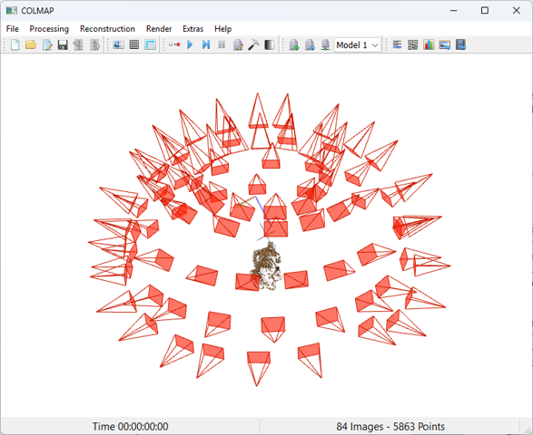
84 Images - 5863 Points
This means all 84 images were successfully registered, resulting in a sparse reconstruction with 5,863 3D points.
Figure 6. COLMAP GUI displaying the sparse point cloud and camera poses.
Optional: Run the full pipeline using a batch script
You can automate the entire COLMAP pipeline with a batch file. A sample .bat script containing all the commands described above is available at:
scripts/run_colmap_adjusted.bat
Before running the script, make sure to update the paths to match your local setup.
Reference results
The reference COLMAP output, including the sparse point cloud and estimated camera poses, is available in the sample dataset repository: datasets/plush-dog.
Notes on parameter tuning and dataset quality
Note: The parameters used in this tutorial were selected to produce reliable results for the sample dataset. They are not optimized for performance or accuracy and are not intended as general-purpose defaults. For other datasets, you may need to adjust the values based on your reconstruction goals, such as speed, completeness, or visual quality. Finding the right configuration often requires several iterations.
Advanced users can also bypass COLMAP’s internal feature extraction and matching by injecting custom features or correspondences directly into the COLMAP database. This allows you to integrate learned feature pipelines or third-party tools while still using COLMAP for mapping.
In some cases, collecting a more complete or higher-quality dataset is more effective than adjusting reconstruction parameters. However, this is not always possible. For example:
The dataset may be captured in uncontrolled environments
Lighting, texture, or camera settings may not be under your control
The scene may have large textureless areas or reflective surfaces
In such cases, parameter tuning becomes essential to compensate for limitations in the input data.
1.4 - Train the 3D Gaussian Model Using gsplat
To train the 3D Gaussian Splatting model, run the following commands:
Replace <GSPLAT_REPOSITORY_FOLDER> with the path to your cloned gsplat repository.
Also update <DATA_PATH> and <OUTPUT_PATH> with the correct paths on your local system.
Parameter reference
default: Uses the default configuration profile in simple_trainer.py
--eval_steps -1: Disables evaluation during training
--disable_viewer: Disables the built-in Nerfstudio viewer
--data_factor 4: Downsamples input images by a factor of 4
--save_ply: Enables saving the output model in PLY format
--ply_steps 30000: Saves the .ply file at training step 30,000
--data_dir: Path to the dataset directory (same as used in COLMAP)
--result_dir: Output folder for training results
Expected output
If training starts successfully, you will see a progress bar. Upon completion, the output will include a message like:
In the example above, training took approximately 12 minutes on the system described in the tested setup. The resulting model contains 167,459 Gaussians. The final .ply file is saved at:
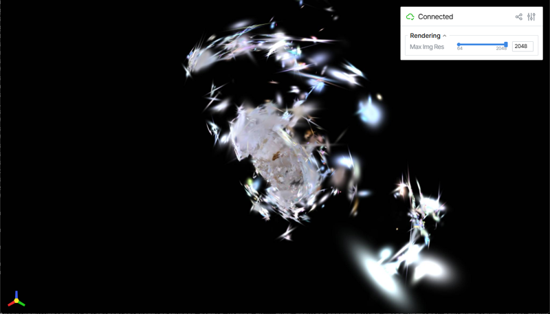
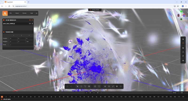
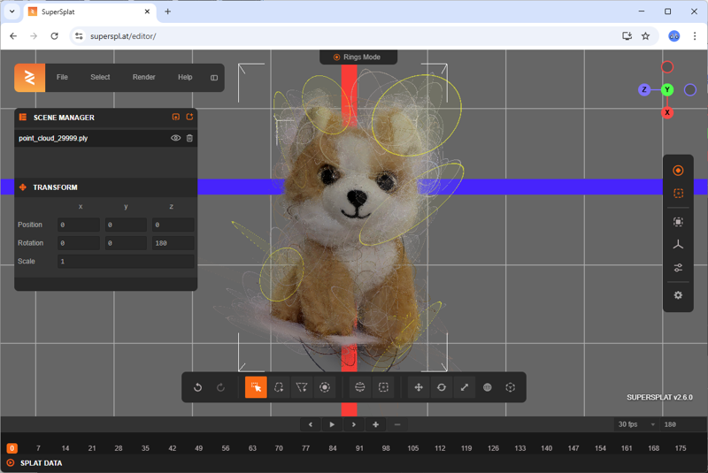
The viewer renders the trained Gaussian Splatting model. Floating artifacts often appear around the main object. The next section, Edit a 3D Gaussian Splatting Model in SuperSplat, shows how to clean and post-process the model for better visualization or downstream use.
Floating artifacts in the Gaussian Splatting model, rendered in the gsplat viewer. These artifacts typically surround the scene before cleanup.
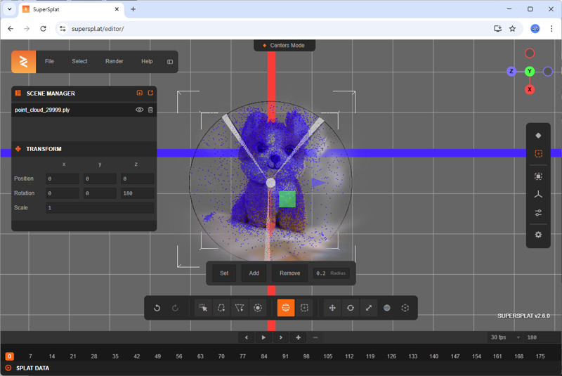
The reconstructed plush toy appears at the center of the same scene when viewed up close.
1.5 - Edit a 3D Gaussian Splatting Model in SuperSplat
After training and exporting the .ply file, you can open the model in SuperSplat Editor for visual inspection and manual refinement.
Common editing tasks include:
Removing floating artifacts or unwanted background Gaussians
The following suggestions can help improve reconstruction quality and workflow efficiency:
Capture more images when possible. Larger datasets improve reconstruction robustness, even if they require more cleanup or processing time.
Experiment with tool parameters. Adjusting settings in COLMAP and gsplat can significantly affect results.
Document parameter choices. Keeping track of parameters helps ensure reproducibility and improves future runs.
Use image downsampling for faster training. Use higher --data_factor values (for example, 4) during testing to reduce memory and speed up training. For best quality, train final models on high-resolution inputs.
Notes on the example dataset
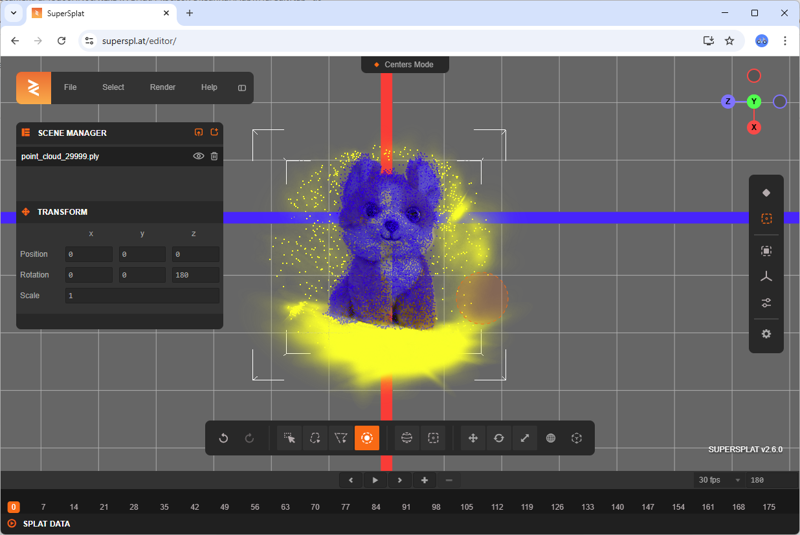
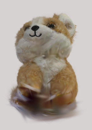
This tutorial’s dataset was captured mostly from dome-like camera angles, covering only the upper hemisphere of the object. As a result, the bottom of the model appears incomplete when viewed from below.
Model view from below, showing sparse Gaussians and an incomplete surface.
For many use cases, such as turntable demos or frontal visualizations, this coverage is sufficient.
However, for fully enclosed 3D models, you should capture additional images from lower angles.
If the object is rigid, consider placing it on its side to photograph the underside. Make sure there is sufficient overlap with other views to maintain alignment.
Approximate time per stage
The table below summarizes typical time requirements for each stage in the pipeline:
Step
Approximate Time
Capturing images
20 minutes
Processing images in COLMAP
1 minute
Training a model in gsplat
12 minutes
Editing in SuperSplat
10 minutes
Note: COLMAP time reflects only a successful reconstruction run. Parameter tuning and retries can add significant time depending on the dataset.
Frequently asked questions
Note: These answers apply primarily to object- or tabletop-scale capture, as demonstrated in this tutorial. Outdoor scenes or large-scale environments may require different tools, workflows, and parameter settings.
Can I use a smartphone camera?
Yes. While this tutorial used an interchangeable-lens camera, modern smartphones can produce similar results if lighting is adequate and images are sharp and stable.
Should I take photos or record video?
Photos are preferred due to better control over focus and exposure. Video can work if shot at 60 FPS or higher with minimal blur.
How many images do I need?
For small objects, 100–250 images is usually enough. Full 360° coverage may require more.
Can I use zoom, autofocus, or auto exposure?
Try to avoid them. Use manual focus and a fixed focal length to maintain consistent camera intrinsics for more accurate pose estimation.
Do I need to capture all sides of the object?
Not always. For turntable-style outputs, upper and side coverage may be enough. For full 360° models, also capture the underside.
Does the object need to have texture?
Yes, ideally. Surfaces with visible patterns, edges, or textures improve feature matching. Flat, shiny, or textureless objects are harder to reconstruct.
Can I use a textured background to help?
Yes, but keep in mind:
COLMAP may rely on the background for pose estimation
Reconstruction quality on the object itself may still be limited
You may need extra cleanup to isolate the object afterward